Chapter 5 Handling projections and coordinate systems
5.1 Projections and coordinate systems
Even well-seasoned GIS analysts can stumble over projections and coordinate systems.
A projection is simply a mathematical function for transforming the X and Y coordinates of a point in one spatial reference framework to X and Y coordinates in a different spatial reference framework.
Initially, any point on the earth can have its location specified by the degrees north or south of the equator (latitude) and west or east of the Greenwich meridian (longitude). These spherical coordinates can be transformed to Cartesian coordinates using tried and true projection transformation equations. For the geodesically inclined, see Snyder’s comprehensive work, Map Projections–A working Manual.
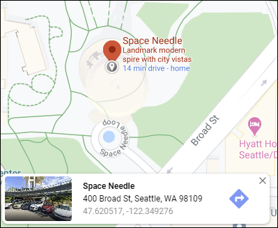
For example, the Space Needle shows up in Google Maps at (-122.349276°, 47.620517°)
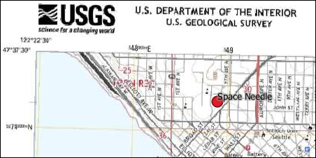
The same location on the USGS topographic sheet indicates tick marks for both UTM and State Plane coordinates. For the same location on the earth’s surface, the WA State Plane North HARN coordinates are (1266575.4, 230021.7) ft, and the UTM Zone 10 N coordinates are (548894.1, 5274326.9) m.
BONUS Why would you use a Cartesian projected coordinate reference system versus a geographic (latitude/longitude) reference system?
5.2 On-the-fly projection in desktop GIS
How is it that we could not see the ZIP code outlines in our R map (Chapter @(export)) when they appeared just fine in QGIS? Desktop GIS applications including ArcMap and QGIS employ “on-the-fly” projection. The software will read any existing coordinate reference system (CRS) tags associated with a data set (e.g., a .prj file as part of a shape file or a “world file” accompanying a TIFF or JPEG file). The software will transform the coordinates of the data to match the CRS of other data in the same map viewer. This process does not alter data in any way, but rather just changes display properties.
On-the-fly projection for mapping is highly convenient, particularly if you have many different data sets that originated from different agencies, each of which uses a different CRS standard. For example, some products from the USGS are referenced to latitude/longitude and some are referenced to UTM; the City of Seattle and King County uses WA State Plane North and the Washington State Departments of Transportation and Natural Resources uses WA State Plane South.
However, there is a dark side. Although the layers appear to register correctly, any analyses performed between layers will not produce correct results. This is because the geoprocessing algorithms use the absolute numerical values of the coordinates as if they were drawn on a sheet of graph paper, without respect to whether those coordinates represent any particular CRS. For this reason, any for project involving GIS analysis using multiple data sources, the first step should be to decide on a single CRS and transform all data as necessary to be stored in that CRS.
Which CRS to use will depend on which distortion you want to minimize: area, shape, distance, or direction. See the USGS Map Projections poster for details, which are beyond the scope of this workshop.
5.3 Defining a data set’s coordinate reference system
If you have a sf spatial data frame consisting of vector data or a raster data set (covered in Chapter @(raster)) that is not tagged with its CRS, there are simple commands to do so: st_crs() for sf data frames and crs() for rasters. The function can be used to show the current CRS or to (re)define the CRS. The CRS can be specified in one of two ways, using EPSG codes, which uses numerical codes for different CRSs, or a prj4 string, which verbosely lists all the parameters for a given CRS. Using EPSG codes is more convenient than using prj4 strings.
If you obtain a spatial data set, one of the things you need to be absolutely certain of is its CRS. Most data sets are provided with either files (e.g., .prj files for shape files) or internal metadata (e.g., embedded in a GeoTIFF), or at least a description of their CRS. If you do not know the CRS of your data, you can make educated guesses.
In any case if you have a data set that has no CRS defined, although it may not be absolutely necessary, you should define its CRS in order to follow best practices.
Let’s redo the exercise from Chapter @(points) in which we created the Space Needle point, but not include the CRS:
snxy <- data.frame(name = "Space Needle", x = -122.3493, y = 47.6205)
space_needle <- st_as_sf(snxy, coords = c("x", "y"))
When we look at its CRS, it shows NA:
st_crs(space_needle)## Coordinate Reference System: NABecause we knew in advance that these coordinates were stored in WGS84 (EPSG 4326), we can now set the data frame’s CRS:
st_crs(space_needle) <- 4326
st_crs(space_needle)
## Coordinate Reference System:
## User input: EPSG:4326
## wkt:
## GEOGCRS["WGS 84",
## DATUM["World Geodetic System 1984",
## ELLIPSOID["WGS 84",6378137,298.257223563,
## LENGTHUNIT["metre",1]]],
## PRIMEM["Greenwich",0,
## ANGLEUNIT["degree",0.0174532925199433]],
## CS[ellipsoidal,2],
## AXIS["geodetic latitude (Lat)",north,
## ORDER[1],
## ANGLEUNIT["degree",0.0174532925199433]],
## AXIS["geodetic longitude (Lon)",east,
## ORDER[2],
## ANGLEUNIT["degree",0.0174532925199433]],
## USAGE[
## SCOPE["Horizontal component of 3D system."],
## AREA["World."],
## BBOX[-90,-180,90,180]],
## ID["EPSG",4326]]Note that setting the data frame’s CRS does not change any coordinate XY values, it is only metadata.
If you want a list of EPSG codes and their descriptions and proj4 values, use the rgdal package’s make_EPSG function. For example what if we wanted the EPSG code for UTM Zone 10 N …
epsg <- make_EPSG()
utm10 <- epsg[grep("UTM.*10", epsg$note),]
kable(utm10) %>% kable_styling(bootstrap_options = "striped", full_width = F, position = "left")| code | note | prj4 | prj_method | |
|---|---|---|---|---|
| 2099 | 26710 | NAD27 / UTM zone 10N | +proj=utm +zone=10 +datum=NAD27 +units=m +no_defs +type=crs | Transverse Mercator |
| 2267 | 26910 | NAD83 / UTM zone 10N | +proj=utm +zone=10 +datum=NAD83 +units=m +no_defs +type=crs | Transverse Mercator |
| 3109 | 3157 | NAD83(CSRS) / UTM zone 10N | +proj=utm +zone=10 +ellps=GRS80 +units=m +no_defs +type=crs | Transverse Mercator |
| 3376 | 32210 | WGS 72 / UTM zone 10N | +proj=utm +zone=10 +ellps=WGS72 +units=m +no_defs +type=crs | Transverse Mercator |
| 3446 | 32310 | WGS 72 / UTM zone 10S | +proj=utm +zone=10 +south +ellps=WGS72 +units=m +no_defs +type=crs | Transverse Mercator |
| 3516 | 32410 | WGS 72BE / UTM zone 10N | +proj=utm +zone=10 +ellps=WGS72 +units=m +no_defs +type=crs | Transverse Mercator |
| 3586 | 32510 | WGS 72BE / UTM zone 10S | +proj=utm +zone=10 +south +ellps=WGS72 +units=m +no_defs +type=crs | Transverse Mercator |
| 3657 | 32610 | WGS 84 / UTM zone 10N | +proj=utm +zone=10 +datum=WGS84 +units=m +no_defs +type=crs | Transverse Mercator |
| 3735 | 32710 | WGS 84 / UTM zone 10S | +proj=utm +zone=10 +south +datum=WGS84 +units=m +no_defs +type=crs | Transverse Mercator |
| 4233 | 3717 | NAD83(NSRS2007) / UTM zone 10N | +proj=utm +zone=10 +ellps=GRS80 +units=m +no_defs +type=crs | Transverse Mercator |
| 4256 | 3740 | NAD83(HARN) / UTM zone 10N | +proj=utm +zone=10 +ellps=GRS80 +units=m +no_defs +type=crs | Transverse Mercator |
| 5062 | 6339 | NAD83(2011) / UTM zone 10N | +proj=utm +zone=10 +ellps=GRS80 +units=m +no_defs +type=crs | Transverse Mercator |
| 6530 | 6653 | NAD83(CSRS) / UTM zone 10N + CGVD2013 height | +proj=utm +zone=10 +ellps=GRS80 +units=m +vunits=m +no_defs +type=crs | (null) |
… or if we wanted to find out what EPSG code 2927 is:
kable(epsg %>%filter(code == 2927)) %>% kable_styling(bootstrap_options = "striped", full_width = F, position = "left")| code | note | prj4 | prj_method |
|---|---|---|---|
| 2927 | NAD83(HARN) / Washington South (ftUS) | +proj=lcc +lat_0=45.3333333333333 +lon_0=-120.5 +lat_1=47.3333333333333 +lat_2=45.8333333333333 +x_0=500000.0001016 +y_0=0 +ellps=GRS80 +units=us-ft +no_defs +type=crs | Lambert Conic Conformal (2SP) |
5.4 Coordinate transformation
If you have a data set stored in one CRS and you want to transform its coordinates to match another CRS, use st_transform() for sf data frames or the projctRaster() function for raster data sets.
Here we will make a new Space Needle point stored with UTM 10 NAD83. Note the changed coordinates shown in the geometry column.
(space_needle_utm10 <- space_needle %>% st_transform(26910))## Simple feature collection with 1 feature and 1 field
## Geometry type: POINT
## Dimension: XY
## Bounding box: xmin: 548894.1 ymin: 5274327 xmax: 548894.1 ymax: 5274327
## Projected CRS: NAD83 / UTM zone 10N
## name geometry
## 1 Space Needle POINT (548894.1 5274327)Or if you want to overwrite the data of an existing data frame with a new CRS:
(space_needle <- space_needle %>% st_transform(26910))## Simple feature collection with 1 feature and 1 field
## Geometry type: POINT
## Dimension: XY
## Bounding box: xmin: 548894.1 ymin: 5274327 xmax: 548894.1 ymax: 5274327
## Projected CRS: NAD83 / UTM zone 10N
## name geometry
## 1 Space Needle POINT (548894.1 5274327)which should be done with care because it alters the values of an existing data set.
5.5 Conclusion
For any GIS analysis, it is imperative that all input data sets be stored with the same CRS, otherwise the outputs are almost certain to be non-existent or erroneous.
A best practices work flow would be to take a set of layers that are in a variety of CRS and to transform them all to the same CRS and write them all to a single GPKG for further analysis.